Web Analytics Data Warehouse : Google Analytics and Search

In this tutorial, we will see how to create a dashboard for content marketing that relies on SEO (Search Engine Optimization). It will leverage and blend data from Google Analytics (that track traffic on your website) and Google Search Console (how your website perform on Google Search).

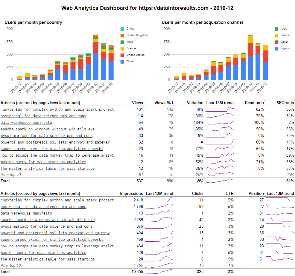
The result will be this Google Sheet dashboard (you can follow the link or see the capture below) which is automatically updated. It’s live from my blog DataIntoResults.com which runs on WordPress but any content marketing platform will do.

This post will encompass many topics: setting the data warehouse and ETL infrastructure, getting the data from Google Analytics and Google Search to the data warehouse, modeling the data so it can be used and setting up a nice dashboard in Google Sheets.

Let’s get started!

What is an web analytics data warehouse?

The first question we need to ask ourselves is what do we want to achieve? The whole point of setting up a web analytics data warehouse is to be able to get custom reports that perfectly suit your need. If not, you could as well use the Google Analytics front end.

Here, I will narrow my interest in two questions: what is relevant to my audience and how to make my articles more SEO-friendly. Nevertheless, this post is designed so you will have plenty of data to focus more on your specific context.

Are my posts relevant to my audience?

Which content is of interest to the audience? I don’t do clickbait, so my articles tend to be long. Therefore, one way to suspect interest is to see how many visitors read the whole article versus those that stop at the beginning. There is this cool feature in Medium called the read ratio (see the capture below). We will make this feature with Google Analytics.

The second metric of interest will be the click through rate (CTR) of the content displayed on Google search. If your content is pushed in front of people but they don’t click, it can be that either your theme is not right or that your title and description is not interesting enough.

Is my content SEO-ready?

Having relevant content is great, but without a way of putting it in front of an audience it’s quite useless. SEO marketing is based on having content in good position for some keywords that people are looking for.

For instance, those day I rank well on the search “postgresql data science” (ranking #1 on DuckDuckGo). This a reasonable keyword combination with traffic and being number one helps to drive visitors.

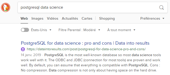
Nevertheless, on overall, the page is on position 27. Digging a bit, I found some keywords combination that are both relevant and with some traffic (opportunities for new content creation).

Setting up the data warehouse infrastructure

Now that we know what we want, we need to spend some time on the infrastructure. You can contact me if you need assistance. Let’s set strong foundations that you will leverage in the future.

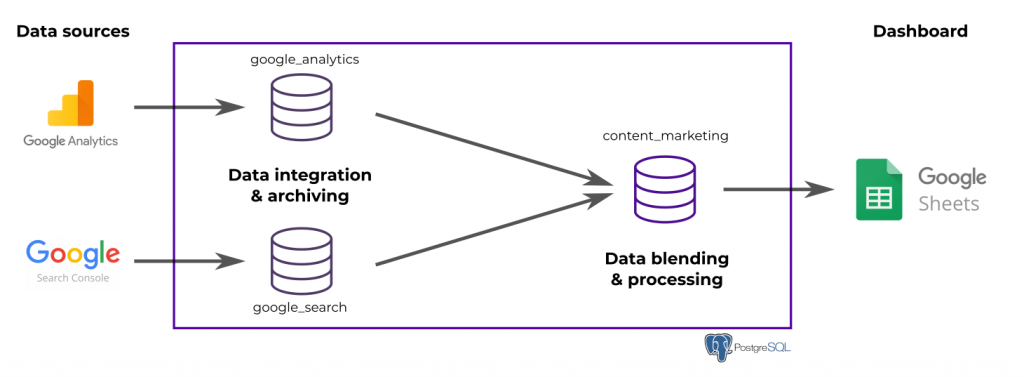
We will use a PostgreSQL data warehouse (open-source) and the Data Brewery ETL (a product of mine, open source as well). PostgreSQL will be where data is stored and processed while Data Brewery will move data from Google services to the database and manage the workflow.

There is two data sources, Google Analytics and Google Search that will be stored inside the PostgreSQL data warehouse (each in a specific module). Then, we will blend them in a new module called content_marketing. At the end, we push the data inside the Google sheet. Nothing too fancy here. We will focus on the modeling part more in details in a next post.

You can find the complete Data Brewery project on GitHub (in the folder v1).

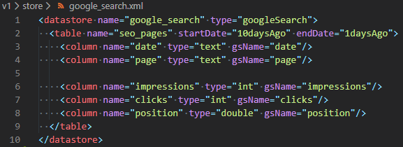
I will not cover the implementation in detail, but the datastore directory contains views on the data sources. For example, below is the datastore for Google Search. It defines a table (virtual) names seo_pages that will contains some information about the last 10 days (how many impressions, clicks and the average position for each page and each day).

The data is then integrated in an archiving module.

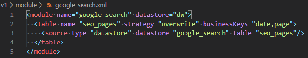
After running the process (using the shell command ipa run-process update), the table google_search.seo_pages will be populated.

The Google Sheets datastore being used to output data, each table is given a SQL query to execute in the data warehouse in order to populate the corresponding area in the Google sheet.

If you want more information on the integration configuration, you can read the Google Analytics, Google Search and Google Sheets documentation pages from Data Brewery.

Modeling the data

Now that we have raw data inside the web analytics data warehouse, we might want to present it nicely in the dashboard. For that, we will leverage the SQL language (how most database speak). In this post, we will keep the work at just making some queries. We will revisit it later to add star schema modeling and make a more proper data warehouse.

First query

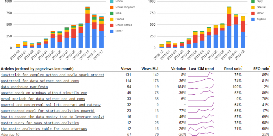
Let’s start with something simple (but far from simplistic), the users per month per country graph.

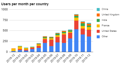
You might see that we limit the number of showed countries to five and we regroup the rest in the Other country. This is important for readability. But you must define how you select the five important countries. It can be a static selection, or it can be dynamic. In this case, I take the 5 biggest countries in the previous month.

As you wee below, the user_country part (the first select) is simple, the rest is only due to the 5 countries selection.

-- Aggregate raw data per month and country
with users_country as (
  select to_char(to_date(date, 'YYYYMMDD'), 'YYYY-MM') as period,
    country, sum(users) as users
  from google_analytics.sessions
  -- Take only the last 13 months (not the current one)
  where to_char(to_date(date, 'YYYYMMDD'), 'YYYY-MM') < to_char(current_date, 'YYYY-MM')
    and to_char(to_date(date, 'YYYYMMDD'), 'YYYY-MM') >= to_char(current_date - interval'13 months', 'YYYY-MM')
  group by 1, 2
),
-- Order the countries by number of users in the previous month
top_countries as (
  select country, row_number() over (order by users desc) as rk
  from users_country
  where period = to_char(current_date - interval'1 month', 'YYYY-MM')
),
-- Select the best performing countries
top_countries_select as (
  select *
  from top_countries
  where rk <= 5
),
-- keep only the best 5 country and affect the rest to Other
reduce_countries as (
  select period,
    coalesce(top_countries_select.country, 'Other') as country, 
    sum(users) as users
  from users_country
  left join top_countries_select using (country) 
  group by 1, 2
)
-- Finish with some ordering
select *
from reduce_countries
order by 1 desc, 3 desc

As you can see in the DATA – Users country sheet, columns A to C are filled by the ETL. On top of that we use a cross table to produce the chart.

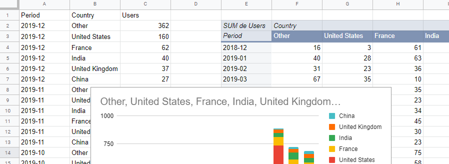
As you can see, it’s not that simple because we want something nice to show, we manipulate raw data and finally because Google Sheet is limiting.

But let’s make some magic.

The read ratio

Remember, the read ratio is the number of visitors that read the whole content piece divided by the number of visitors on this content. The second part is easy as it’s provided by default on Google Analytics.

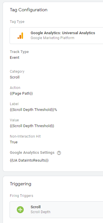
For the first part, the number of visitors that read the article in full, we will use the events mechanism from Google Analytics. I recommend to use Google Tag Manager which allows to configure easily Google Analytics events.

I defined the following tag (see the capture). We will have an event category named Scroll that will be triggered on the page Scroll (I’ve set 25,50,75 and 90%). The parameter {{UA DataIntoResults}} is my Google Analytics view ID.

In the google_analytics.events table we will find those events.

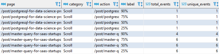
Notice that the action value is the same than the page. This is so because we will use the unique_events columns. If the action is a constant like “Scroll”, unique_event will be counted only one per visits even if the visitor read many posts in full.

Now, place to action, or the SQL query. I want to highlight 3 things:

• Raw data must be cleaned a bit, pages have sometimes parameters. For instance /mypage and /mypage?parameter=1 is not the same page for Google Analytics. Most of the time it’s the same from a business perspective. The code regexp_replace(page, '[?&].*$', '') will clean that (lines 4 and 9).
• We filter the data and keep only what is after 01/15/2020. Scroll tracking was implemented at that date (lines 20 and 29).
• We use the 75% threshold to define an article as read. The proper value depends on your website layout (line 18).

-- Cleaning the pages in events to avoid duplicates
with clean_events as (
  select
    regexp_replace(page, '[?&].*$', '') as clean_page, *
  from google_analytics.events 
),
-- Cleaning the pages in sessions to avoid duplicates
clean_sessions as (
  select regexp_replace(page, '[?&].*$', '') as clean_page, *
  from google_analytics.sessions 
),
-- For each page, how many people read more than 75% ?
-- The Scroll event was implemented on 2020-01-15 so skip 
-- everything before, it is not relevant
end_of_page_events as (
  select clean_page as page, sum(unique_events) as finish_count
  from clean_events
  where label = '75%'
    and category = 'Scroll'
    and date > '20200115'
  group by 1
),
-- For each page track the number of unique pageviews
-- We also just keep view after the implementation date of 
-- scroll tracking.
start_of_page_events as (
  select clean_page as page, sum(unique_pageviews) as start_count
  from clean_sessions
  where date > '20200115'
  group by 1
)
-- Blend those
select page, start_count, finish_count, 
  coalesce(finish_count, 0)*1.0/start_count as read_ratio
from start_of_page_events 
-- It's a left join because some articles are started
-- but were never read up to the 75% mark.
left join end_of_page_events using (page)

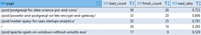
And there we have our read ratio:

Last focus: those sparklines

I’m a big fan of Edward Tufte who invented the term sparkline in his quest of information density. Sparkline provide temporal context without taking to much space.

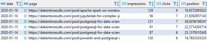
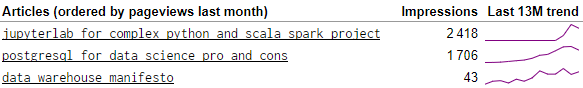
For instance, we use the impression metric (excerpt below) which inform on the number of people that saw each page on Google search. By adding a sparkline for the trend over the last 13 months we provide more value. We can see that while the second article (PostgreSQL for Data Science) raised slowly, the first article (Jupyter for Complex Python and Scala Spark Projects) has gained more impressions quickly. The last one (Data Warehouse Manifesto), doesn’t have a lot of impressions and never had. It is just not a good content for SEO.

Now the sad news is that plotting 13 data points per page require 13 columns which is a bit of pain in SQL. We start by creating a reference table that provide for each month (the last 13 months) their ordering (from 1 to 13). This is done lines 8 to 11. Then, starting line 42 we aggregate data with a condition on the month number. That allows to pivot the data from rows to columns.

-- We avoid page duplication because of page parameters
with clean_sessions as (
  select regexp_replace(page, '[?&].*$', '') as clean_page, *
  from google_analytics.sessions 
),
-- Creating a reference table with the last 13 months and their ordering
weeks_ref as (
  select to_char(ts, 'YYYY-MM') as year_week, 
    row_number() over (order by ts) as rk
  from generate_series(current_date - interval'13 months', 
    current_date - interval'1 months', '1 month') ts
),
-- Unique page view over the last 13 months (up to end of last month)
pages_stats_row as (
  select to_char(to_date(date, 'YYYYMMDD'), 'YYYY-MM') as year_week,    
    clean_page as page, sum(unique_pageviews) as pageviews
  from clean_sessions
  where unique_pageviews > 0
    and to_char(to_date(date, 'YYYYMMDD'), 'YYYY-MM') 
      < to_char(current_date, 'IYYY-MM')
    and to_char(to_date(date, 'YYYYMMDD'), 'YYYY-MM') 
      >= to_char(current_date - interval'13 months', 'IYYY-MM')
  group by 1, 2  
),
-- SEO Data
clean_seo as (
  select to_char(to_date(date, 'YYYY-MM-DD'), 'YYYY-MM') as year_week,
    regexp_replace(page, '^https?://[a-z\.]+', '') as page, 
    sum(impressions) as impressions, sum(clicks) as clicks, 
    sum(impressions*position)/sum(impressions) as position,
    coalesce(sum(clicks),0)*1.0/sum(impressions) as ctr
  from google_search.seo_pages
  where to_char(to_date(date, 'YYYY-MM-DD'), 'YYYY-MM') 
      < to_char(current_date, 'YYYY-MM')
    and to_char(to_date(date, 'YYYY-MM-DD'), 'YYYY-MM') 
      >= to_char(current_date - interval'13 months', 'YYYY-MM')
  group by 1, 2
),
-- Pivot the data
pages_stats as (
  select page,
    coalesce(sum(case when rk = 1 then pageviews end),0) as pageviews_month_1,
    coalesce(sum(case when rk = 2 then pageviews end),0) as pageviews_month_2,
    coalesce(sum(case when rk = 3 then pageviews end),0) as pageviews_month_3,
    coalesce(sum(case when rk = 4 then pageviews end),0) as pageviews_month_4,
    coalesce(sum(case when rk = 5 then pageviews end),0) as pageviews_month_5,
    coalesce(sum(case when rk = 6 then pageviews end),0) as pageviews_month_6,
    coalesce(sum(case when rk = 7 then pageviews end),0) as pageviews_month_7,
    coalesce(sum(case when rk = 8 then pageviews end),0) as pageviews_month_8,
    coalesce(sum(case when rk = 9 then pageviews end),0) as pageviews_month_9,
    coalesce(sum(case when rk = 10 then pageviews end),0) as pageviews_month_10,
    coalesce(sum(case when rk = 11 then pageviews end),0) as pageviews_month_11,
    coalesce(sum(case when rk = 12 then pageviews end),0) as pageviews_month_12,
    coalesce(sum(case when rk = 13 then pageviews end),0) as pageviews_month_13,
    coalesce(sum(case when rk = 1 then impressions end),0) as impressions_month_1,
    coalesce(sum(case when rk = 2 then impressions end),0) as impressions_month_2,
    coalesce(sum(case when rk = 3 then impressions end),0) as impressions_month_3,
    coalesce(sum(case when rk = 4 then impressions end),0) as impressions_month_4,
    coalesce(sum(case when rk = 5 then impressions end),0) as impressions_month_5,
    coalesce(sum(case when rk = 6 then impressions end),0) as impressions_month_6,
    coalesce(sum(case when rk = 7 then impressions end),0) as impressions_month_7,
    coalesce(sum(case when rk = 8 then impressions end),0) as impressions_month_8,
    coalesce(sum(case when rk = 9 then impressions end),0) as impressions_month_9,
    coalesce(sum(case when rk = 10 then impressions end),0) as impressions_month_10,
    coalesce(sum(case when rk = 11 then impressions end),0) as impressions_month_11,
    coalesce(sum(case when rk = 12 then impressions end),0) as impressions_month_12,
    coalesce(sum(case when rk = 13 then impressions end),0) as impressions_month_13,
    coalesce(sum(case when rk = 1 then clicks end),0) as clicks_month_1,
    coalesce(sum(case when rk = 2 then clicks end),0) as clicks_month_2,
    coalesce(sum(case when rk = 3 then clicks end),0) as clicks_month_3,
    coalesce(sum(case when rk = 4 then clicks end),0) as clicks_month_4,
    coalesce(sum(case when rk = 5 then clicks end),0) as clicks_month_5,
    coalesce(sum(case when rk = 6 then clicks end),0) as clicks_month_6,
    coalesce(sum(case when rk = 7 then clicks end),0) as clicks_month_7,
    coalesce(sum(case when rk = 8 then clicks end),0) as clicks_month_8,
    coalesce(sum(case when rk = 9 then clicks end),0) as clicks_month_9,
    coalesce(sum(case when rk = 10 then clicks end),0) as clicks_month_10,
    coalesce(sum(case when rk = 11 then clicks end),0) as clicks_month_11,
    coalesce(sum(case when rk = 12 then clicks end),0) as clicks_month_12,
    coalesce(sum(case when rk = 13 then clicks end),0) as clicks_month_13,
    coalesce(sum(case when rk = 1 then position end),100) as position_month_1,
    coalesce(sum(case when rk = 2 then position end),100) as position_month_2,
    coalesce(sum(case when rk = 3 then position end),100) as position_month_3,
    coalesce(sum(case when rk = 4 then position end),100) as position_month_4,
    coalesce(sum(case when rk = 5 then position end),100) as position_month_5,
    coalesce(sum(case when rk = 6 then position end),100) as position_month_6,
    coalesce(sum(case when rk = 7 then position end),100) as position_month_7,
    coalesce(sum(case when rk = 8 then position end),100) as position_month_8,
    coalesce(sum(case when rk = 9 then position end),100) as position_month_9,
    coalesce(sum(case when rk = 10 then position end),100) as position_month_10,
    coalesce(sum(case when rk = 11 then position end),100) as position_month_11,
    coalesce(sum(case when rk = 12 then position end),100) as position_month_12,
    coalesce(sum(case when rk = 13 then position end),100) as position_month_13
  from pages_stats_row
  left join clean_seo using (year_week, page)
  inner join weeks_ref using (year_week)
  group by 1
)
select pages_stats.*, read_ratio
from pages_stats 
left join content_marketing.read_ratio using (page)

Having now those 13 columns per indicator (pageviews, impressions, clicks and position) for each page (each page being a row), we can draw those little sparklines in Google Sheet.

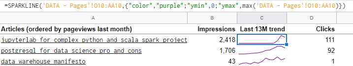
Notice that beside the data point selection, you can pass parameters to control the behavior. You can read more on Sparkline in the Google Sheets documentation.

Initialize and automate refresh

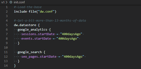
The default configuration looks for the last 10 days from Google Analytics and Google Search. That is obviously not convenient when you have a report that go 13 months in the past (you need to wait 13 months).

Therefore, we will use a init.conf (see below) to bootstrap the data warehouse using ipa run-module -c init.conf update. This will take some times as we grab the last 400 days of data.

Lastly, we want the web analytics data warehouse to be refreshed without human interaction. The easiest way is to use a scheduler, for instance cron under Linux. Below, you can see the command to update the data warehouse every day at 5am UTC.

# m h  dom mon dow   command
0 5 * * * cd ~/dwh/web-analytics-data-warehouse/v1 && ~/app/ipa/bin/ipa run-process update

Our Google Sheet dashboard will therefore be refreshed every day (not much will change from day to day as it’s a monthly report).

Congrats, we have now a fully operational web analytics data warehouse! What would you add to make it more relevant?

Let's stay in touch with the newsletter